Lesson 6: Joining Tables in SQL

Learn how to extract data from multiple tables by joining them.

Estimated Read Time: 4 - 6 Hours

Learning Goals

In this lesson, you will learn to:

Select and execute appropriate join types (INNER, LEFT, FULL OUTER, SELF) based on business requirements and table relationships
Construct multi-table queries by joining 3+ tables following primary key-foreign key relationships
Handle complex join scenarios including self-joins for hierarchical data and multiple joins to the same dimension table
Extract business insights from multi-dimensional data by combining fact tables with dimension tables in large-scale datasets

1. Introduction: The Limitations of Single-Table Analysis

Throughout the first five lessons of this module, you have developed a solid foundation in SQL fundamentals. You can extract specific columns from tables, filter data using sophisticated WHERE clauses, sort results meaningfully, and calculate aggregate metrics that inform business decisions. These are substantial achievements, and they represent the core competencies that every data analyst must possess.

However, there is a fundamental limitation to everything you have accomplished thus far: you have been working exclusively with single tables. In the real world of business intelligence and data analysis, this constraint renders approximately 80% of meaningful business questions unanswerable. Consider the following scenarios that a data analyst at Northwind Traders might encounter on a typical workday:

“Which customers have generated the most revenue for our company this quarter?”
“What is our total sales performance broken down by product category?”
“Which suppliers provide the products that contribute most significantly to our profit margins?”
“How do sales territories compare in terms of revenue generation, and which employees are responsible for managing our highest-performing regions?”
“Which products in our inventory have never been ordered, representing potential dead stock?”

Each of these questions — and thousands like them — requires information that exists across multiple tables in the Northwind database. Customer names reside in the customers table, while order values live in the order_details table. Product information is stored separately from the categories to which those products belong. Employee data is distinct from the territories they manage and the orders they process.

This architectural decision is not accidental or arbitrary. It reflects one of the fundamental principles of relational database design: normalization. Rather than duplicating information across multiple locations (which would create maintenance nightmares and consistency problems), relational databases store each piece of information in exactly one place and use relationships to connect related data across tables.

This is where SQL joins become essential. Joins are the mechanism through which we reassemble normalized data to answer comprehensive business questions. They allow us to combine rows from two or more tables based on related columns, creating unified result sets that provide complete pictures of business activities.

Mastering joins represents a pivotal moment in your development as a data analyst. It is the point at which you transition from being able to answer simple, single-dimensional questions to tackling complex, multi-faceted business intelligence challenges. By the end of this lesson, you will possess the skills necessary to navigate the intricate web of relationships within any relational database and extract precisely the insights that business stakeholders require.

2. Understanding Table Relationships: The Foundation of Joins

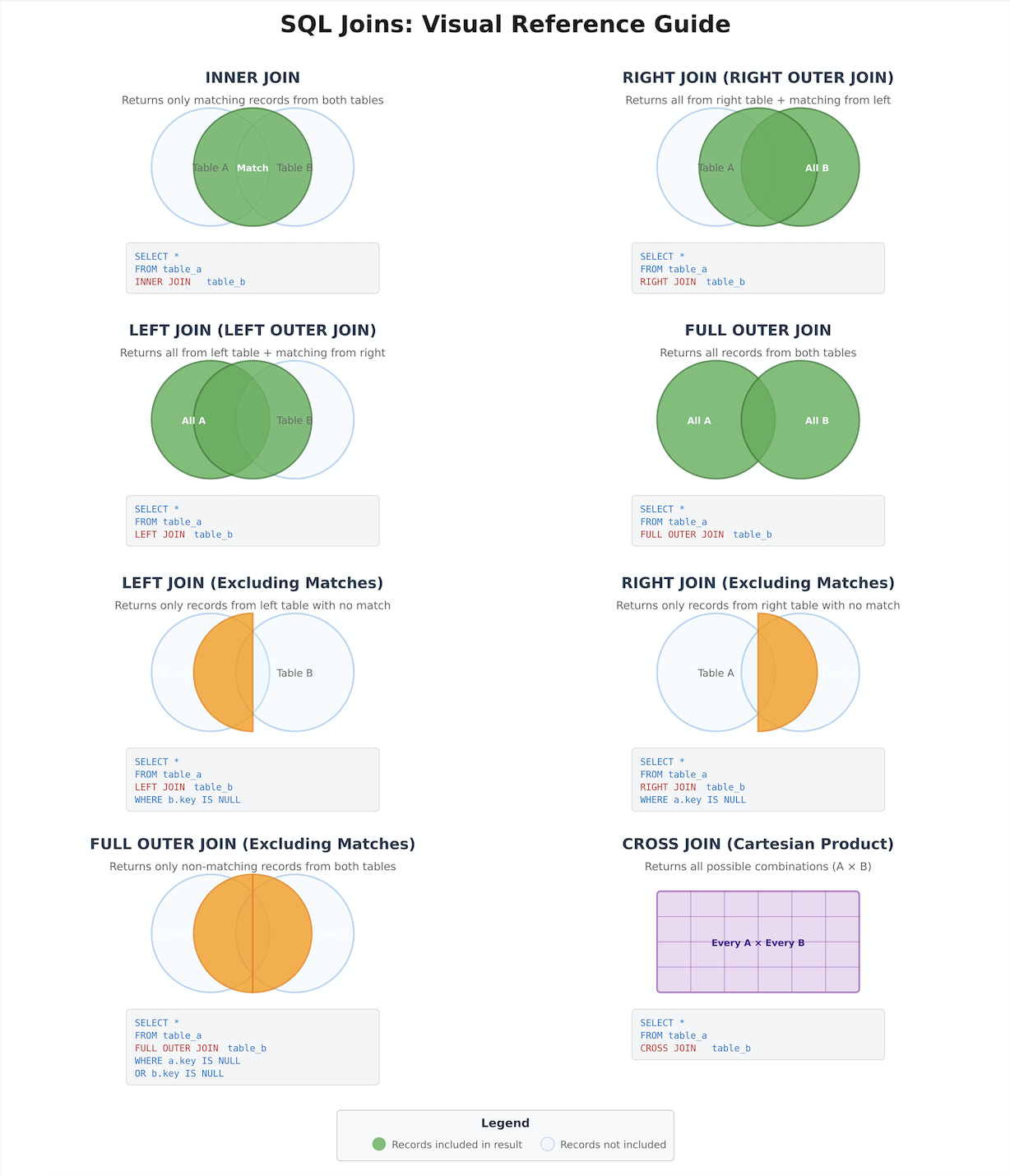
Before we explore the syntax and mechanics of different join types, we must first develop a conceptual understanding of how tables relate to one another within the Northwind database. Every successful join operation relies on identifying and leveraging these relationships correctly. Consider Figure 1 below that shows a comprehensive visual guide showing all SQL join types as Venn diagrams. The diagram includes:

INNER JOIN – Only matching records (intersection)
LEFT JOIN – All from left + matches from right
RIGHT JOIN – All from right + matches from left
FULL OUTER JOIN – All records from both tables
LEFT JOIN (Excluding) – Only left table records with no match
RIGHT JOIN (Excluding) – Only right table records with no match
FULL OUTER JOIN (Excluding) – Non-matching records from both
CROSS JOIN – All possible combinations (Cartesian product)

2.1. Primary Keys and Foreign Keys

You were introduced to the concepts of primary keys and foreign keys in Lesson 2, but now we must examine them through the lens of their critical role in enabling joins.

A primary key is a column (or combination of columns) that uniquely identifies each row in a table. In the customers table, for example, customer_id serves as the primary key. Every customer has a unique identifier, and no two customers share the same customer_id value. This uniqueness is enforced by database constraints, ensuring data integrity at the structural level.

A foreign key is a column in one table that references the primary key of another table. In the orders table, the customer_id column is a foreign key that references the primary key in the customers table. This establishes a relationship: each order is associated with exactly one customer, but each customer may have multiple orders.

This is known as a one-to-many relationship, and it is the most common relationship type you will encounter in relational databases. The “one” side is the table containing the primary key (customers), and the “many” side is the table containing the foreign key (orders).

2.2. Visualizing Northwind’s Relationship Network

The Northwind database contains an intricate network of related tables. Understanding these relationships is crucial for constructing effective joins. Let us examine some of the key relationship paths:

The Customer Order Journey:

				
					customers (customer_id) [Primary Key]
    ↓ one-to-many
orders (customer_id [Foreign Key], order_id [Primary Key])
    ↓ one-to-many
order_details (order_id [Foreign Key], product_id [Foreign Key])
    ↓ many-to-one
products (product_id [Primary Key], category_id [Foreign Key], supplier_id [Foreign Key])
    ↓ many-to-one
categories (category_id [Primary Key])
suppliers (supplier_id [Primary Key])

This relationship chain allows us to answer questions like: “Which customers purchased products from the Beverages category?” Such a question requires joining five tables together, following the foreign key references from customers through to categories.

The Employee Territory Structure:

				
					employees (employee_id [Primary Key], reports_to [Foreign Key to employees])
    ↓ one-to-many
employee_territories (employee_id [Foreign Key], territory_id [Foreign Key])
    ↓ many-to-one
territories (territory_id [Primary Key], region_id [Foreign Key])
    ↓ many-to-one
regions (region_id [Primary Key])

This structure enables questions about organizational hierarchy and geographical sales performance.

The Shipping Relationship:

				
					orders (order_id [Primary Key], shipper_id [Foreign Key])
    ↓ many-to-one
shippers (shipper_id [Primary Key])

This simple relationship allows us to analyze shipping costs and carrier performance.

2.3. The Join Condition: Establishing the Connection

When we write a join operation in SQL, we must explicitly tell the database how to match rows from one table with rows from another. This is accomplished through the join condition, which typically takes the form of equating a foreign key in one table to the corresponding primary key in another table.

For example, to join the orders table with the customers table, we would use the condition:

				
					orders.customer_id = customers.customer_id

This tells the database: “For each row in the orders table, find the row in the customers table where the customer_id values match, and combine those rows into a single result row.”

Understanding this fundamental principle is essential because every join you write will follow this pattern: identify the relationship, locate the key columns, and specify the matching condition.

3. The INNER JOIN: Finding Matching Records

The INNER JOIN is the most frequently used join type in data analysis, and it represents the foundation upon which understanding all other join types is built. An INNER JOIN returns only those rows where a match exists in both tables according to the specified join condition.

3.1. Business Context: When to Use INNER JOIN

An INNER JOIN is appropriate whenever you need to combine data from related tables and you are only interested in records that have corresponding entries in both tables. This is the natural choice for most analytical queries because it focuses on actual business activity rather than theoretical possibilities.

Consider this business question: “What is the total revenue generated by each customer?” This question implicitly assumes that we are only interested in customers who have actually placed orders. Customers who exist in our database but have never purchased anything are irrelevant to this particular analysis. An INNER JOIN between customers and orders is therefore the appropriate choice.

3.2. INNER JOIN Syntax and Structure

The basic syntax for an INNER JOIN follows this pattern:

				
					SELECT 
    columns_from_both_tables
FROM table1
INNER JOIN table2
    ON table1.key_column = table2.key_column;

Let us examine a concrete example that answers a common business question.

Business Case: Customer Order Summary

The sales department needs a report showing customer names alongside their order information. This requires combining data from the customers table (which contains customer names and contact information) with the orders table (which contains order dates and identifiers).

				
					-- Retrieve customer names with their order dates
-- Purpose: Allow sales team to see customer purchase activity
SELECT 
    c.company_name,
    c.contact_name,
    o.order_id,
    o.order_date,
    o.shipped_date
FROM customers c
INNER JOIN orders o 
    ON c.customer_id = o.customer_id
ORDER BY c.company_name, o.order_date DESC;

Let us analyze this query component by component:

Table Aliases: We use c as an alias for customers and o as an alias for orders. This is a professional standard that improves readability and reduces typing, particularly when dealing with multiple joins.
Column Qualification: Each column in the SELECT clause is prefixed with its table alias (c.company_name, o.order_id). This is technically optional when column names are unique across tables, but it is considered best practice because it makes the query’s logic explicit and prevents errors when tables share column names.
The Join Condition: ON c.customer_id = o.customer_id establishes the relationship. For each customer, the database will find all matching orders and create result rows combining information from both tables.
Ordering Results: The results are sorted by company name alphabetically, and within each company, orders are sorted from most recent to oldest.

This query will return only customers who have placed at least one order. Any customer in the database who has never ordered anything will not appear in the results, because there would be no matching row in the orders table.

3.3. Multiple Column Joins and Filtering

INNER JOINs become more powerful when combined with WHERE clauses and aggregate functions. Consider this more sophisticated business question:

Business Case: High-Value German Customers

Management wants to identify customers in Germany who have generated significant revenue, defined as total purchases exceeding €10,000. This information will be used to prioritize account management resources.

				
					-- Identify high-value customers in Germany for VIP treatment
-- Combines customer data, orders, and order details to calculate revenue
SELECT 
    c.company_name,
    c.contact_name,
    c.city,
    COUNT(DISTINCT o.order_id) AS total_orders,
    SUM(od.unit_price * od.quantity * (1 - od.discount)) AS total_revenue
FROM customers c
INNER JOIN orders o 
    ON c.customer_id = o.customer_id
INNER JOIN order_details od 
    ON o.order_id = od.order_id
WHERE c.country = 'Germany'
GROUP BY c.company_name, c.contact_name, c.city
HAVING SUM(od.unit_price * od.quantity * (1 - od.discount)) > 10000
ORDER BY total_revenue DESC;

This query demonstrates several advanced techniques:

Chained Joins: We join three tables in sequence: customers → orders → order_details. Each join builds upon the previous one, following the relationship path through the database.
Revenue Calculation: The formula od.unit_price * od.quantity * (1 – od.discount) calculates the actual revenue for each line item, accounting for discounts applied to the order.
WHERE for Pre-Aggregation Filtering: The WHERE c.country = ‘Germany’ filter is applied before grouping, limiting our analysis to German customers only.
HAVING for Post-Aggregation Filtering: The HAVING clause filters the grouped results, showing only customers whose total revenue exceeds €10,000.
DISTINCT in COUNT: Using COUNT(DISTINCT o.order_id) ensures we count unique orders, even though each order may contain multiple line items in order_details.

3.4. INNER JOIN with Multiple Conditions

Sometimes the relationship between tables requires more than one condition to establish a match. While this is less common with well-designed normalized databases, it is worth understanding.

				
					-- Example: Join based on multiple conditions
SELECT 
    p.product_name,
    od.unit_price AS order_price,
    p.unit_price AS catalog_price
FROM products p
INNER JOIN order_details od 
    ON p.product_id = od.product_id 
    AND p.unit_price = od.unit_price
WHERE od.unit_price != p.unit_price;

This query would find cases where the price charged on an order differs from the current catalog price, which might indicate price changes over time or special discounts.

4. The LEFT JOIN: Including Non-Matching Records

While INNER JOINs serve the majority of analytical needs, there are critical business scenarios where we need to include records even when matches do not exist in the related table. This is where the LEFT JOIN (also called LEFT OUTER JOIN) becomes essential.

4.1. Business Context: When to Use LEFT JOIN

A LEFT JOIN returns all rows from the left (first) table and matching rows from the right (second) table. When no match exists, the result will still include the row from the left table, but columns from the right table will contain NULL values.

This is particularly valuable for questions like:

“Which customers have never placed an order?” (finding gaps in activity)
“Which products have never been sold?” (identifying dead inventory)
“Which territories have no assigned employees?” (finding coverage gaps)

The key distinction is that these questions explicitly seek to identify the absence of relationships, not their presence.

4.2. LEFT JOIN Syntax and Structure

				
					SELECT 
    columns_from_both_tables
FROM table1
LEFT JOIN table2
    ON table1.key_column = table2.key_column;

The critical principle: ALL rows from table1 will appear in the results, regardless of whether matches exist in table2.

Business Case: Identifying Inactive Customers

The marketing team wants to run a re-engagement campaign targeting customers who have accounts in the system but have never placed an order. These are potential customers who expressed initial interest (by registering) but never converted to actual sales.

				
					-- Find customers who have never placed an order
-- Purpose: Target dormant accounts for re-engagement campaigns
SELECT 
    c.customer_id,
    c.company_name,
    c.contact_name,
    c.city,
    c.country,
    c.phone
FROM customers c
LEFT JOIN orders o 
    ON c.customer_id = o.customer_id
WHERE o.order_id IS NULL
ORDER BY c.country, c.city;

Let us analyze the key components:

LEFT JOIN Logic: This join ensures that every customer appears in the result set. If a customer has orders, those orders will be joined. If a customer has no orders, the customer row will still appear, but all columns from the orders table will be NULL.
The Crucial WHERE Clause: WHERE o.order_id IS NULL filters the results to show only rows where no match was found in the orders table. We check for NULL in order_id because it is the primary key of the orders table and would never be NULL in an actual order record.
Business Value: This query directly enables business action. The marketing team can export this list and create targeted campaigns with messaging like “We miss you!” or “Complete your first order and save 15%.”

4.3. LEFT JOIN for Complete Inventory Analysis

Business Case: Product Sales Performance Including Unsold Items

The inventory manager needs a comprehensive report showing all products along with their sales performance. This must include products that have never been ordered, as these represent potential overstock or obsolescence issues.

				
					-- Complete product sales analysis including items with zero sales
-- Helps identify slow-moving or dead inventory
SELECT 
    p.product_id,
    p.product_name,
    c.category_name,
    s.company_name AS supplier,
    p.unit_price AS catalog_price,
    p.units_in_stock,
    p.discontinued,
    COUNT(od.order_id) AS times_ordered,
    COALESCE(SUM(od.quantity), 0) AS total_units_sold,
    COALESCE(SUM(od.unit_price * od.quantity * (1 - od.discount)), 0) AS total_revenue
FROM products p
INNER JOIN categories c 
    ON p.category_id = c.category_id
INNER JOIN suppliers s 
    ON p.supplier_id = s.supplier_id
LEFT JOIN order_details od 
    ON p.product_id = od.product_id
GROUP BY 
    p.product_id, 
    p.product_name, 
    c.category_name, 
    s.company_name,
    p.unit_price,
    p.units_in_stock,
    p.discontinued
ORDER BY total_revenue DESC, p.product_name;

This query demonstrates sophisticated join combinations:

Mixed Join Types: We use INNER JOINs for categories and suppliers because every product must have a category and supplier (enforced by foreign key constraints). We use a LEFT JOIN for order_details because we specifically want to include products that have never been ordered.
COALESCE Function: COALESCE(SUM(od.quantity), 0) handles NULL values gracefully. For products with no orders, SUM(od.quantity) would return NULL, which COALESCE converts to 0. This makes the report more readable and prevents confusion.
Comprehensive Business Insight: This single query provides inventory managers with complete visibility into product performance, allowing them to identify both bestsellers and products that may need to be discontinued or promoted more aggressively.

4.4. Finding Gaps with LEFT JOIN

A particularly powerful pattern with LEFT JOINs is identifying records that exist in one table but not in another:

				
					-- Find all categories that currently have no products
-- Indicates either data quality issues or category obsolescence
SELECT 
    c.category_id,
    c.category_name,
    c.description
FROM categories c
LEFT JOIN products p 
    ON c.category_id = p.category_id
WHERE p.product_id IS NULL;

This pattern—LEFT JOIN followed by WHERE checking for NULL in the right table—is a standard technique for finding gaps, missing relationships, and orphaned records.

5. The RIGHT JOIN: A Mirror Perspective

The RIGHT JOIN (or RIGHT OUTER JOIN) is the conceptual inverse of the LEFT JOIN. It returns all rows from the right (second) table and matching rows from the left (first) table, with NULLs filling in when no match exists.

5.1. Why RIGHT JOIN Exists (and Why It Is Rarely Used)

In practice, RIGHT JOINs are used far less frequently than LEFT JOINs, for a simple reason: any RIGHT JOIN can be rewritten as a LEFT JOIN by reversing the table order. Most SQL practitioners prefer to standardize on LEFT JOINs for consistency and readability.

However, understanding RIGHT JOIN is important because:

You will encounter it in queries written by others
It provides conceptual completeness in understanding join operations
In some specific query structures, it may be more readable than reordering tables

5.2. RIGHT JOIN Syntax

				
					SELECT 
    columns_from_both_tables
FROM table1
RIGHT JOIN table2
    ON table1.key_column = table2.key_column;

This returns all rows from table2, with matching rows from table1 where they exist.

Example: Products with Their Orders (Right Join Perspective)

				
					-- Show all orders with product information
-- Uses RIGHT JOIN to ensure all orders appear
SELECT 
    o.order_id,
    o.order_date,
    p.product_name,
    od.quantity,
    od.unit_price
FROM products p
RIGHT JOIN order_details od 
    ON p.product_id = od.product_id
RIGHT JOIN orders o 
    ON od.order_id = o.order_id
ORDER BY o.order_date DESC;

This could be more naturally written using LEFT JOINs by starting with orders:

				
					-- Same query using LEFT JOIN (preferred style)
SELECT 
    o.order_id,
    o.order_date,
    p.product_name,
    od.quantity,
    od.unit_price
FROM orders o
LEFT JOIN order_details od 
    ON o.order_id = od.order_id
LEFT JOIN products p 
    ON od.product_id = p.product_id
ORDER BY o.order_date DESC;

Best Practice Recommendation

Default to using LEFT JOINs and arrange your FROM clause so that the table you want complete results from appears first. Reserve RIGHT JOIN for situations where reversing the table order would make the query significantly less readable.

6. The FULL OUTER JOIN: Complete Coverage

A FULL OUTER JOIN (or FULL JOIN) returns all rows from both tables, matching them where possible and filling with NULLs where matches do not exist. This is the most comprehensive join type, ensuring that no data from either table is excluded from the results.

6.1. Business Context: When to Use FULL OUTER JOIN

FULL OUTER JOINs are used less frequently than INNER or LEFT JOINs, but they are valuable in specific scenarios:

Comparing two datasets to find differences and similarities
Data quality audits to identify mismatches
Reconciliation processes
Comprehensive gap analysis

6.2. FULL OUTER JOIN Syntax

				
					SELECT 
    columns_from_both_tables
FROM table1
FULL OUTER JOIN table2
    ON table1.key_column = table2.key_column;

6.3. Business Case: Product-Supplier Reconciliation

Imagine that Northwind maintains a separate tracking system for supplier relationships, and you need to reconcile it with the actual products in inventory to find discrepancies.

				
					-- Reconcile products with supplier contracts
-- Find products without suppliers and suppliers without products
SELECT 
    COALESCE(p.product_id, 'No Product') AS product_id,
    COALESCE(p.product_name, 'No Product') AS product_name,
    COALESCE(s.company_name, 'No Supplier') AS supplier_name,
    CASE 
        WHEN p.product_id IS NULL THEN 'Supplier has no products'
        WHEN s.supplier_id IS NULL THEN 'Product has no supplier'
        ELSE 'Matched'
    END AS reconciliation_status
FROM products p
FULL OUTER JOIN suppliers s 
    ON p.supplier_id = s.supplier_id
WHERE p.product_id IS NULL 
   OR s.supplier_id IS NULL
ORDER BY reconciliation_status, supplier_name;

This query identifies:

Suppliers in the system with no associated products (potential data cleanup targets)
Products with no supplier (data integrity violations)

The CASE statement categorizes each row, making the discrepancies immediately actionable for the data governance team.

7. The SELF JOIN: Tables Relating to Themselves

A SELF JOIN is not a different type of join operation; rather, it is the technique of joining a table to itself. This is necessary when a table contains hierarchical or recursive relationships, where rows relate to other rows within the same table.

7.1. Business Context: Organizational Hierarchies

The most common use case for SELF JOINs in Northwind is the employee table, which contains a hierarchical reporting structure. Each employee has a reports_to column that contains the employee_id of their manager, who is also an employee in the same table.

7.2. Business Case: Employee Organizational Chart

The HR department needs a report showing employees alongside their managers for an organizational chart.

				
					-- Create employee-manager relationship report
-- Shows organizational hierarchy for HR and management
SELECT 
    e.employee_id,
    e.first_name || ' ' || e.last_name AS employee_name,
    e.title AS employee_title,
    m.first_name || ' ' || m.last_name AS manager_name,
    m.title AS manager_title
FROM employees e
LEFT JOIN employees m 
    ON e.reports_to = m.employee_id
ORDER BY m.employee_id, e.last_name;

Critical observations:

Two Aliases for Same Table: We reference the employees table twice, using aliases e (for employee) and m (for manager). This is essential because we need to distinguish between the employee rows and the manager rows.
LEFT JOIN Reasoning: We use LEFT JOIN rather than INNER JOIN because the top-level executive (the CEO or president) has no manager. An INNER JOIN would exclude this person from the results.
String Concatenation: The || operator combines first and last names with a space to create full names. This is a PostgreSQL-specific syntax; other databases use different concatenation methods.

7.3. Business Case: Finding Direct Reports

Conversely, management might want to see which employees report directly to a specific manager:

				
					-- Find all employees who report directly to Nancy Davolio (employee_id = 1)
-- Useful for managers to see their team members
SELECT 
    e.employee_id,
    e.first_name || ' ' || e.last_name AS employee_name,
    e.title,
    e.hire_date
FROM employees e
WHERE e.reports_to = 1
ORDER BY e.hire_date;

This is actually a simpler query that doesn’t require a join at all, but understanding the SELF JOIN concept helps us recognize when we might need to expand this to show multiple levels of the hierarchy.

8. The CROSS JOIN: Cartesian Products

A CROSS JOIN produces the Cartesian product of two tables, meaning every row from the first table is combined with every row from the second table. If table1 has 10 rows and table2 has 5 rows, a CROSS JOIN will produce 50 rows (10 × 5).

8.1. Business Context: When to Use CROSS JOIN

CROSS JOINs have legitimate use cases, though they are rare in typical data analysis:

Generating all possible combinations (e.g., every product with every supplier for pricing analysis)
Creating calendar templates (every day with every time slot)
Statistical sampling or scenario analysis

Warning:

CROSS JOINs can produce extremely large result sets very quickly. Be cautious when using them on large tables.

8.2. CROSS JOIN Syntax

				
					SELECT 
    columns_from_both_tables
FROM table1
CROSS JOIN table2;

8.3. Business Case: Product-Category Analysis Matrix

A product manager wants to analyze potential new product opportunities by examining all possible product-category combinations:

				
					-- Generate all possible product-category combinations
-- For strategic product line expansion analysis
SELECT 
    c.category_name,
    s.company_name AS supplier_name,
    s.city AS supplier_city,
    s.country AS supplier_country
FROM categories c
CROSS JOIN suppliers s
WHERE s.country IN ('USA', 'UK', 'Germany')
ORDER BY c.category_name, s.company_name;

This creates a matrix showing every category paired with every supplier from key markets, which can help identify gaps in the product portfolio (e.g., “We have no suppliers in the USA for Condiments”).

Important Note: In practice, CROSS JOINs are often written using the older comma syntax:

				
					-- Older syntax (still valid)
SELECT c.category_name, s.company_name
FROM categories c, suppliers s;

However, the explicit CROSS JOIN syntax is preferred in modern SQL because it makes the intention clear and prevents accidental Cartesian products from forgotten join conditions.

9. Multiple Joins: Connecting Complex Data Paths

Real-world business questions frequently require joining three, four, or even more tables together. The key to managing this complexity is understanding the relationship path and constructing joins methodically, one table at a time.

9.1. Strategy for Multi-Table Joins

When faced with a question requiring multiple joins:

Identify the Starting Point: Determine which table contains the primary subject of your analysis
Map the Relationship Path: Trace the foreign key connections from your starting table to your destination
Build Incrementally: Add one join at a time and verify the logic before proceeding
Use Clear Aliases: Meaningful table aliases make complex queries readable
Comment Your Intentions: Add comments explaining the business logic

9.2. Business Case: Comprehensive Order Analysis

The executive team wants a detailed report showing customer names, employee names who processed the orders, product details, categories, and suppliers for all orders in a specific date range.

				
					-- Comprehensive order report with all related dimensions
-- Links customers, employees, products, categories, and suppliers
-- Used for executive quarterly business reviews
SELECT 
    -- Customer Information
    c.company_name AS customer,
    c.city AS customer_city,
    c.country AS customer_country,
    
    -- Order Information
    o.order_id,
    o.order_date,
    o.shipped_date,
    
    -- Employee Information
    e.first_name || ' ' || e.last_name AS sales_representative,
    
    -- Product Information
    p.product_name,
    cat.category_name,
    
    -- Supplier Information
    s.company_name AS supplier,
    
    -- Financial Details
    od.quantity,
    od.unit_price,
    od.discount,
    (od.unit_price * od.quantity * (1 - od.discount)) AS line_total
    
FROM orders o

-- Join customer information
INNER JOIN customers c 
    ON o.customer_id = c.customer_id

-- Join employee (sales representative) information
INNER JOIN employees e 
    ON o.employee_id = e.employee_id

-- Join order details (line items)
INNER JOIN order_details od 
    ON o.order_id = od.order_id

-- Join product information
INNER JOIN products p 
    ON od.product_id = p.product_id

-- Join category information
INNER JOIN categories cat 
    ON p.category_id = cat.category_id

-- Join supplier information
INNER JOIN suppliers s 
    ON p.supplier_id = s.supplier_id

-- Filter to specific date range
WHERE o.order_date BETWEEN '1997-01-01' AND '1997-12-31'

-- Sort for readability
ORDER BY o.order_date DESC, c.company_name, p.product_name;

This query joins seven tables together, following these relationship paths:

orders → customers (via customer_id)
orders → employees (via employee_id)
orders → order_details (via order_id)
order_details → products (via product_id)
products → categories (via category_id)
products → suppliers (via supplier_id)

9.3. Performance Considerations for Multiple Joins

While modern database systems are optimized to handle complex joins efficiently, there are practical considerations:

Join Order Matters for Readability: While the database optimizer will determine the actual execution order, arranging joins logically helps humans understand the query.
Filter Early: Apply WHERE conditions as early as possible to reduce the working dataset.
Use Appropriate Join Types: Don’t use LEFT JOIN when INNER JOIN is sufficient, as it may require more processing.
Index Key Columns: Ensure foreign key and primary key columns are properly indexed (usually handled automatically, but worth verifying for performance-critical queries).

10. Choosing the Right Join Type: A Decision Framework

Selecting the appropriate join type is a critical skill that directly impacts the accuracy and relevance of your analysis. Here is a systematic framework for making this decision:

10.1. Decision Tree

Question 1: Do I need to preserve all rows from one or both tables?

No → Use INNER JOIN
Yes, from one table → Proceed to Question 2
Yes, from both tables → Use FULL OUTER JOIN

Question 2: Which table’s rows must all be preserved?

The first table (left side) → Use LEFT JOIN
The second table (right side) → Use RIGHT JOIN (or rewrite as LEFT JOIN)

Question 3: Am I looking for missing relationships?

Yes → Use LEFT JOIN with WHERE checking for NULL in the right table

Question 4: Do I need every possible combination?

Yes → Use CROSS JOIN (rare, be cautious)

Question 5: Does the table relate to itself?

Yes → Use SELF JOIN with appropriate alias strategy

10.3. Practical Examples of Join Selection

Business Question	Appropriate Join Type	Reasoning
“Show me all customers and their orders”	INNER JOIN	Only interested in customers who have ordered
“Show me all customers, including those who haven’t ordered”	LEFT JOIN	Must preserve all customers
“Which products have never been sold?”	LEFT JOIN with WHERE NULL check	Looking for missing relationships
“Match every employee with every territory for planning”	CROSS JOIN	Need all combinations
“Show employees and their managers”	SELF JOIN	Hierarchical relationship within one table
“Find discrepancies between two inventory systems”	FULL OUTER JOIN	Need to see mismatches in both directions

11. Common Join Mistakes and How to Avoid Them

Even experienced analysts make mistakes with joins. Understanding common pitfalls will help you avoid them and debug problems when they arise.

11.1. Mistake 1: Forgetting the Join Condition

				
					-- WRONG: Missing ON clause creates accidental CROSS JOIN
SELECT c.company_name, o.order_id
FROM customers c
INNER JOIN orders o;
-- This will create a Cartesian product!

Fix: Always include an explicit ON clause specifying the join condition.

				
					-- CORRECT:
SELECT c.company_name, o.order_id
FROM customers c
INNER JOIN orders o ON c.customer_id = o.customer_id;

11.2. Mistake 2: Using the Wrong Join Type

				
					-- WRONG: Using INNER JOIN when you want to include products with no orders
SELECT p.product_name, COUNT(od.order_id) AS times_ordered
FROM products p
INNER JOIN order_details od ON p.product_id = od.product_id
GROUP BY p.product_name;
-- Products never ordered won't appear!

Fix: Use LEFT JOIN to preserve all products.

				
					-- CORRECT:
SELECT p.product_name, COUNT(od.order_id) AS times_ordered
FROM products p
LEFT JOIN order_details od ON p.product_id = od.product_id
GROUP BY p.product_name
ORDER BY times_ordered DESC;

11.3. Mistake 3: Ambiguous Column Names

				
					-- WRONG: Which customer_id are we selecting?
SELECT customer_id, company_name, order_date
FROM customers
INNER JOIN orders ON customers.customer_id = orders.customer_id;
-- Error: column reference "customer_id" is ambiguous

Fix: Always qualify column names with table aliases, especially in joins.

				
					-- CORRECT:
SELECT c.customer_id, c.company_name, o.order_date
FROM customers c
INNER JOIN orders o ON c.customer_id = o.customer_id;

11.4. Mistake 4: Incorrect Filtering in LEFT JOIN

				
					-- WRONG: WHERE clause on right table converts LEFT JOIN to INNER JOIN
SELECT c.company_name, o.order_date
FROM customers c
LEFT JOIN orders o ON c.customer_id = o.customer_id
WHERE o.order_date > '1997-01-01';
-- This excludes customers with no orders!

Fix: Move conditions on the right table to the ON clause, or use OR IS NULL.

				
					-- CORRECT (if you want to filter):
SELECT c.company_name, o.order_date
FROM customers c
LEFT JOIN orders o 
    ON c.customer_id = o.customer_id 
    AND o.order_date > '1997-01-01';

-- Or filter only the left table:
SELECT c.company_name, o.order_date
FROM customers c
LEFT JOIN orders o ON c.customer_id = o.customer_id
WHERE c.country = 'USA';

11.5. Mistake 5: Duplicate Rows from One-to-Many Relationships

				
					-- PROBLEM: Each customer appears multiple times (once per order)
SELECT c.company_name, c.city, o.order_id
FROM customers c
INNER JOIN orders o ON c.customer_id = o.customer_id;
-- Returns 830 rows because customers have multiple orders

Understanding: This is not necessarily a mistake—it depends on what you are trying to achieve. If you want one row per order, this is correct. If you want one row per customer, you need aggregation.

				
					-- If you want one row per customer with order count:
SELECT 
    c.company_name, 
    c.city,
    COUNT(o.order_id) AS total_orders
FROM customers c
INNER JOIN orders o ON c.customer_id = o.customer_id
GROUP BY c.company_name, c.city;

11.6. Mistake 6: Joining on Non-Key Columns Without Understanding

				
					-- DANGEROUS: Joining on non-unique columns
SELECT p1.product_name, p2.product_name
FROM products p1
INNER JOIN products p2 ON p1.unit_price = p2.unit_price
WHERE p1.product_id != p2.product_id;
-- This finds products with the same price, which may or may not be intentional

Consideration: Joining on non-key columns can be valid (finding duplicates, matching by attributes), but ensure you understand the cardinality and expected results.

12. Best Practices for Professional Join Queries

As you develop proficiency with joins, adopting professional standards will make your queries more maintainable, readable, and reliable.

12.1. Always Use Explicit JOIN Syntax

Avoid the older implicit join syntax:

				
					-- OLD STYLE (avoid):
SELECT c.company_name, o.order_id
FROM customers c, orders o
WHERE c.customer_id = o.customer_id;

Prefer the explicit JOIN syntax:

				
					-- MODERN STYLE (preferred):
SELECT c.company_name, o.order_id
FROM customers c
INNER JOIN orders o ON c.customer_id = o.customer_id;

The explicit syntax makes the join type and conditions clear, reducing errors and improving readability.

12.2. Use Meaningful Table Aliases

Choose aliases that are intuitive and consistent:

				
					-- GOOD: Clear, standard abbreviations
FROM customers c
INNER JOIN orders o ON c.customer_id = o.customer_id
INNER JOIN order_details od ON o.order_id = od.order_id

-- AVOID: Cryptic or inconsistent aliases
FROM customers x1
INNER JOIN orders tbl2 ON x1.customer_id = tbl2.customer_id

12.3. Format for Readability

Adopt a consistent formatting style that makes complex queries scannable:

				
					-- Well-formatted multi-join query
SELECT 
    c.company_name,
    e.first_name || ' ' || e.last_name AS employee,
    o.order_date,
    p.product_name,
    od.quantity,
    od.unit_price * od.quantity AS line_total
FROM orders o
INNER JOIN customers c 
    ON o.customer_id = c.customer_id
INNER JOIN employees e 
    ON o.employee_id = e.employee_id
INNER JOIN order_details od 
    ON o.order_id = od.order_id
INNER JOIN products p 
    ON od.product_id = p.product_id
WHERE o.order_date BETWEEN '1997-01-01' AND '1997-12-31'
ORDER BY o.order_date DESC, c.company_name;

12.4. Comment Complex Joins

For queries with intricate logic or non-obvious business rules, include explanatory comments:

				
					-- Revenue analysis excluding discontinued products and cancelled orders
-- Used for monthly executive reporting
-- Last updated: 2024-01-15 by Data Analytics Team

SELECT 
    cat.category_name,
    SUM(od.unit_price * od.quantity * (1 - od.discount)) AS revenue
FROM categories cat
INNER JOIN products p 
    ON cat.category_id = p.category_id
INNER JOIN order_details od 
    ON p.product_id = od.product_id
INNER JOIN orders o 
    ON od.order_id = o.order_id
WHERE 
    p.discontinued = 0  -- Active products only
    AND o.shipped_date IS NOT NULL  -- Exclude unshipped (potentially cancelled) orders
    AND o.order_date >= CURRENT_DATE - INTERVAL '1 month'
GROUP BY cat.category_name
ORDER BY revenue DESC;

5. Test Incrementally

When building complex multi-table joins, test each join addition:

				
					-- Step 1: Start with base table
SELECT * FROM orders WHERE order_date > '1997-01-01';

-- Step 2: Add first join
SELECT o.*, c.company_name 
FROM orders o
INNER JOIN customers c ON o.customer_id = c.customer_id
WHERE o.order_date > '1997-01-01';

-- Step 3: Add second join
SELECT o.*, c.company_name, od.product_id, od.quantity
FROM orders o
INNER JOIN customers c ON o.customer_id = c.customer_id
INNER JOIN order_details od ON o.order_id = od.order_id
WHERE o.order_date > '1997-01-01';

-- Continue building...

12.6. Understand Row Multiplication

Be aware that joins can multiply rows based on relationship cardinality:

A customer with 5 orders joined to order_details will produce many rows (one per line item per order)
Use aggregation when you need to collapse back to one row per entity
Use DISTINCT cautiously—it can mask underlying data issues

12.7. Verify Join Conditions

Always verify that your join conditions match the actual foreign key relationships in the database schema. Joining on incorrect columns can produce subtle errors that are difficult to debug.

13. Performance Optimization for Joins

While PostgreSQL’s query optimizer handles much of the performance tuning automatically, understanding basic optimization principles will help you write more efficient queries.

13.1. Indexes and Join Performance

Joins rely heavily on indexes for performance. The database uses indexes to quickly locate matching rows rather than scanning entire tables.

Key columns that should be indexed:

Primary keys (automatically indexed)
Foreign keys (should be indexed, though not always automatic)
Columns frequently used in WHERE clauses
Columns frequently used in ORDER BY clauses

You can verify indexes on a table:

				
					-- Check indexes on the orders table
SELECT 
    tablename, 
    indexname, 
    indexdef
FROM pg_indexes
WHERE tablename = 'orders';

13.2. Filter Early and Aggressively

Reduce the dataset size before joining when possible:

				
					-- LESS EFFICIENT: Join first, filter later
SELECT c.company_name, o.order_id
FROM customers c
INNER JOIN orders o ON c.customer_id = o.customer_id
WHERE c.country = 'USA' AND o.order_date > '1997-01-01';

-- MORE EFFICIENT: Filter in subqueries (though modern optimizers may handle both similarly)
SELECT c.company_name, o.order_id
FROM 
    (SELECT * FROM customers WHERE country = 'USA') c
INNER JOIN 
    (SELECT * FROM orders WHERE order_date > '1997-01-01') o
    ON c.customer_id = o.customer_id;

However, modern PostgreSQL query optimizers are sophisticated enough to push predicates down automatically in most cases, so explicit subqueries for filtering are often unnecessary.

13.3. Avoid SELECT *

Request only the columns you need:

				
					-- LESS EFFICIENT:
SELECT *
FROM customers c
INNER JOIN orders o ON c.customer_id = o.customer_id;

-- MORE EFFICIENT:
SELECT c.company_name, c.city, o.order_id, o.order_date
FROM customers c
INNER JOIN orders o ON c.customer_id = o.customer_id;

This reduces the amount of data transferred and processed.

13.4. Use EXPLAIN to Understand Query Execution

PostgreSQL provides the EXPLAIN command to show how a query will be executed:

				
					EXPLAIN
SELECT c.company_name, COUNT(o.order_id) AS order_count
FROM customers c
INNER JOIN orders o ON c.customer_id = o.customer_id
GROUP BY c.company_name;

The output shows the execution plan, including:

Which indexes are used
The order of join execution
Estimated costs and row counts

For more detailed analysis, use EXPLAIN ANALYZE, which actually executes the query and shows real runtime statistics:

				
					EXPLAIN ANALYZE
SELECT c.company_name, COUNT(o.order_id) AS order_count
FROM customers c
INNER JOIN orders o ON c.customer_id = o.customer_id
GROUP BY c.company_name;

Note: Be cautious with EXPLAIN ANALYZE on queries that modify data (INSERT, UPDATE, DELETE), as it will actually execute those modifications.

14. Real-World Business Scenarios: Comprehensive Examples

To solidify your understanding of joins, let us work through a few comprehensive business scenarios that you might encounter as a data analyst at Northwind Traders.

Scenario 1: Sales Analysis

Business Question: “Sales wants to identify customers who have placed more than 5 orders. They want to see the order count along with the earliest and most recent order dates.”

Analysis Approach:

Consider the video walkthrough to understand how to approach this problem.

Video 1 – Answer Sales Analysis question using SQL Joins

Scenario 2: Monthly Sales Performance by Employee

Business Question: “Management wants to see each employee’s sales performance for the last quarter, including total orders processed, total revenue generated, and the number of unique customers served. The report should show employee names, titles, and be sorted by revenue descending.”

Analysis Approach:

Start with employees (we want all employees, even those with no sales)
Join to orders (via employee_id)
Join to order_details to calculate revenue
Aggregate by employee
Format results for executive presentation

				
					-- Quarterly Employee Sales Performance Report
-- Purpose: Evaluate sales team performance for bonuses and reviews
-- Period: Last complete quarter

SELECT 
    -- Employee identification
    e.employee_id,
    e.first_name || ' ' || e.last_name AS employee_name,
    e.title,
    
    -- Performance metrics
    COUNT(DISTINCT o.order_id) AS orders_processed,
    COUNT(DISTINCT o.customer_id) AS unique_customers,
    COUNT(DISTINCT od.product_id) AS unique_products_sold,
    SUM(od.quantity) AS total_units_sold,
    ROUND(SUM(od.unit_price * od.quantity * (1 - od.discount))::numeric, 2) AS total_revenue,
    ROUND(AVG(od.unit_price * od.quantity * (1 - od.discount))::numeric, 2) AS avg_line_item_value
    
FROM employees e

-- Left join to include employees with no sales
LEFT JOIN orders o 
    ON e.employee_id = o.employee_id
    AND o.order_date >= DATE_TRUNC('quarter', CURRENT_DATE - INTERVAL '3 months')
    AND o.order_date < DATE_TRUNC('quarter', CURRENT_DATE)

-- Join order details to calculate revenue
LEFT JOIN order_details od 
    ON o.order_id = od.order_id

-- Group by employee
GROUP BY 
    e.employee_id,
    e.first_name,
    e.last_name,
    e.title

-- Sort by performance
ORDER BY total_revenue DESC NULLS LAST, orders_processed DESC;

Key Insights from This Query:

LEFT JOIN ensures employees with no sales still appear (important for identifying underperformers)
Date filtering in the JOIN ON clause preserves all employees while limiting orders to the relevant period
NULLS LAST ensures employees with no sales appear at the bottom
Multiple metrics provide comprehensive performance view
ROUND function ensures currency values are displayed with two decimal places

Scenario 3: Product Profitability Analysis by Category

Business Question: “The product management team wants to identify which product categories generate the highest profit margins and which categories might need pricing adjustments. Include the number of unique products per category, total units sold, average sale price vs. list price, and calculate estimated profit margins.”

				
					-- Product Category Profitability Analysis
-- Compares actual selling prices to list prices by category
-- Identifies pricing opportunities and margin compression

SELECT 
    c.category_name,
    COUNT(DISTINCT p.product_id) AS products_in_category,
    COUNT(DISTINCT p.product_id) FILTER (WHERE p.discontinued = 0) AS active_products,
    
    -- Sales volume metrics
    SUM(od.quantity) AS total_units_sold,
    COUNT(DISTINCT od.order_id) AS orders_containing_category,
    
    -- Pricing analysis
    ROUND(AVG(p.unit_price)::numeric, 2) AS avg_list_price,
    ROUND(AVG(od.unit_price)::numeric, 2) AS avg_actual_sale_price,
    ROUND(AVG(od.discount)::numeric, 3) AS avg_discount_rate,
    
    -- Revenue calculations
    ROUND(SUM(od.unit_price * od.quantity)::numeric, 2) AS gross_revenue,
    ROUND(SUM(od.unit_price * od.quantity * od.discount)::numeric, 2) AS total_discounts,
    ROUND(SUM(od.unit_price * od.quantity * (1 - od.discount))::numeric, 2) AS net_revenue,
    
    -- Profit margin estimate (assuming 40% cost of goods sold)
    ROUND(SUM(od.unit_price * od.quantity * (1 - od.discount) * 0.60)::numeric, 2) AS estimated_gross_profit,
    ROUND((SUM(od.unit_price * od.quantity * (1 - od.discount) * 0.60) / 
           NULLIF(SUM(od.unit_price * od.quantity * (1 - od.discount)), 0) * 100)::numeric, 2) AS estimated_margin_percent

FROM categories c

INNER JOIN products p 
    ON c.category_id = p.category_id

LEFT JOIN order_details od 
    ON p.product_id = od.product_id

GROUP BY c.category_id, c.category_name

ORDER BY net_revenue DESC;

Advanced Techniques Demonstrated:

FILTER clause for conditional aggregation (counting active vs. discontinued products)
NULLIF to prevent division by zero errors
Nested arithmetic for complex financial calculations
Multiple levels of aggregation (units, orders, revenue, profit)
Estimated profit margin calculation based on business assumption

Scenario 4: Customer Segmentation and Lifetime Value

Business Question: “The marketing team wants to segment customers into tiers based on their purchasing behavior for a targeted retention campaign. Classify customers as VIP (>$10,000 lifetime value), Regular ($1,000-$10,000), or Occasional (<$1,000), and show their purchase frequency and last order date.”

				
					-- Customer Lifetime Value Analysis and Segmentation
-- Identifies customer tiers for targeted marketing campaigns
-- Includes recency, frequency, and monetary value (RFM analysis basis)

SELECT 
    -- Customer identification
    c.customer_id,
    c.company_name,
    c.contact_name,
    c.city,
    c.country,
    
    -- RFM metrics
    COUNT(DISTINCT o.order_id) AS total_orders,
    SUM(od.quantity) AS total_units_purchased,
    MAX(o.order_date) AS last_order_date,
    CURRENT_DATE - MAX(o.order_date) AS days_since_last_order,
    
    -- Financial metrics
    ROUND(SUM(od.unit_price * od.quantity * (1 - od.discount))::numeric, 2) AS lifetime_value,
    ROUND(AVG(od.unit_price * od.quantity * (1 - od.discount))::numeric, 2) AS avg_order_line_value,
    
    -- Customer segmentation
    CASE 
        WHEN SUM(od.unit_price * od.quantity * (1 - od.discount)) >= 10000 THEN 'VIP'
        WHEN SUM(od.unit_price * od.quantity * (1 - od.discount)) >= 1000 THEN 'Regular'
        ELSE 'Occasional'
    END AS customer_tier,
    
    -- Engagement status
    CASE 
        WHEN MAX(o.order_date) >= CURRENT_DATE - INTERVAL '30 days' THEN 'Active'
        WHEN MAX(o.order_date) >= CURRENT_DATE - INTERVAL '90 days' THEN 'Recent'
        WHEN MAX(o.order_date) >= CURRENT_DATE - INTERVAL '180 days' THEN 'Lapsed'
        ELSE 'Inactive'
    END AS engagement_status

FROM customers c

LEFT JOIN orders o 
    ON c.customer_id = o.customer_id

LEFT JOIN order_details od 
    ON o.order_id = od.order_id

GROUP BY 
    c.customer_id,
    c.company_name,
    c.contact_name,
    c.city,
    c.country

-- Focus on customers with at least one order for retention campaign
HAVING COUNT(o.order_id) > 0

ORDER BY lifetime_value DESC;

Business Application: This query enables sophisticated marketing strategies:

VIP customers receive premium service and exclusive offers
Regular customers get loyalty programs to encourage upgrades to VIP
Occasional customers receive re-engagement campaigns
Engagement status determines communication frequency and urgency

Summary

This comprehensive lesson has equipped you with one of the most critical skills in SQL and data analysis: the ability to join tables effectively. Let us recap the essential concepts you have mastered:

1. INNER JOIN: Returns only matching records from both tables. Use this when you need to analyze relationships that actually exist (customers who have orders, products that have been sold).
2. LEFT JOIN: Returns all records from the left table and matching records from the right. Use this when you need to preserve all records from your primary subject table, even when relationships don’t exist (all customers including those with no orders).
3. RIGHT JOIN: Returns all records from the right table and matching records from the left. Rarely used; most queries can be rewritten as LEFT JOINs for consistency.
4. FULL OUTER JOIN: Returns all records from both tables, with NULLs where matches don’t exist. Use for reconciliation and comprehensive gap analysis.
5. SELF JOIN: Joining a table to itself, essential for hierarchical relationships like employee-manager structures.
6. CROSS JOIN: Creates all possible combinations of rows. Use cautiously for specific analytical needs like scenario modeling.

Suggested References

The AI Evolution of Graph Search at Netflix: From Structured Queries to Natural Language

Exercise: SQL Joins

Using the NYC Yellow Taxi Trip Dataset

Exercise Set Overview

These exercises use the NYC Taxi and Limousine Commission’s Yellow Taxi trip data. You’ll be analyzing real-world transportation data to answer business questions that taxi fleet managers, city planners, and operations teams face daily.

Database Schema Reference:

fact_yellow_trips_raw_2025 – Main trip records table
dim_taxi_zones – Location information (pickup/dropoff zones)
dim_rate_codes – Rate code descriptions
dim_payment_types – Payment method descriptions
dim_vendors – Vendor/provider information
dim_date – Date dimension for time-based analysis

Important:

For each of the tasks below:

write the appropriate query to extract information from the database
generate insights and answer the business question

Exercise 1: Basic Taxi Operations Analysis (INNER JOIN)

Business Question: “The NYC Taxi & Limousine Commission wants a report showing trips with pickup and dropoff zone names. Show the first 1,000 trips from January 2025 with vendor names, pickup/dropoff zones, trip distance, and total fare.”

Business Context

Operations managers need to understand trip patterns across different zones to optimize taxi deployment and identify high-demand areas.

Tables Needed

fact_yellow_trips_raw_2025
dim_taxi_zones (twice – for pickup and dropoff)
dim_vendors

Expected Columns

vendor_name
pickup_datetime
pickup_zone
pickup_borough
dropoff_zone
dropoff_borough
trip_distance
total_amount

Skills Needed and Hints

Multiple joins to the same table (taxi_zones for pickup AND dropoff)
Table aliasing for clarity
Date filtering
LIMIT for large datasets
Hint: You’ll need to join dim_taxi_zones twice using different aliases (e.g., pickup_zone and dropoff_zone)

Exercise 2: Payment Method Analysis (LEFT JOIN)

Business Question: “Analyze payment preferences across all payment types. Show all payment methods including those that might not have been used in January 2025, with total transactions and revenue for each.”

Challenge: Explain why cash trips have zero tip amounts while credit card trips have tip data.

Business Context

The finance team wants to understand payment method adoption and identify if any payment types are becoming obsolete.

Tables Needed

dim_payment_types
fact_yellow_trips_raw_2025

Expected Columns

payment_type_desc
total_trips
total_revenue
avg_fare_amount
avg_tip_amount (note: only credit cards have tip data)

Skills Needed and Hints

LEFT JOIN to preserve all payment types
Handling NULL values with COALESCE
Aggregation with GROUP BY
Understanding data patterns (cash vs. credit card tips)

Exercise 3: Zone Coverage Analysis (FULL OUTER JOIN)

Business Question: “Identify zones that are only used for pickups (never dropoffs) or only dropoffs (never pickups) during peak hours (7-9 AM) in January 2025. This helps identify one-directional demand patterns.”

Bonus: Calculate the imbalance ratio (pickups – dropoffs) / (pickups + dropoffs)

Business Context

Fleet managers need to understand if certain zones have imbalanced demand (people only leaving or only arriving), which affects taxi repositioning strategies.

Tables Needed

dim_taxi_zones
fact_yellow_trips_raw_2025 (for pickups)
fact_yellow_trips_raw_2025 (for dropoffs)

Expected Columns

zone_name
borough
pickup_count
dropoff_count
imbalance_status (e.g., “Pickup Only”, “Dropoff Only”, “Balanced”)

Skills Needed and Hints

FULL OUTER JOIN concepts
Subqueries or CTEs for aggregation
CASE statements for categorization
Temporal filtering

Exercise 4: Multi-Dimensional Trip Analysis

Business Question: “Create a comprehensive analysis showing trips by vendor, rate code, and payment type for weekend trips in January 2025. Include trip count, average distance, average fare, and total revenue for each combination.”

Business Context

Revenue management teams need to understand how different pricing structures (rate codes) perform across vendors and payment types to optimize pricing strategies.

Tables Needed

fact_yellow_trips_raw_2025
dim_vendors
dim_rate_codes
dim_payment_types
dim_date

Expected Columns

vendor_name
rate_code_desc
payment_type_desc
trip_count
avg_trip_distance
avg_fare_amount
total_revenue
avg_trip_duration_minutes

Skills Needed and Hints

Multiple dimension table joins
Complex aggregation
Date dimension usage
Calculated fields (trip duration from pickup/dropoff timestamps)

Formula hints:

Trip duration: EXTRACT(EPOCH FROM (tpep_dropoff_datetime – tpep_pickup_datetime)) / 60
Revenue: SUM(total_amount)

Exercise 5: Borough-to-Borough Trip Matrix

Business Question: “Create a trip flow matrix showing the number of trips and average fare between each pair of boroughs (e.g., Manhattan to Brooklyn, Queens to Manhattan, etc.). Identify the top 10 highest-volume borough pairs.”

Business insight: This reveals commuter patterns, tourist movements, and can inform surge pricing strategies.

Business Context

Urban planners and transportation authorities need to understand inter-borough travel patterns to plan infrastructure investments and optimize taxi availability.

Tables Needed

fact_yellow_trips_raw_2025
dim_taxi_zones (for pickup borough)
dim_taxi_zones (for dropoff borough)

Expected Columns

pickup_borough
dropoff_borough
trip_count
avg_fare
avg_distance
total_revenue

Skills Needed and Hints

Self-referencing dimension tables
Aggregation with multiple grouping dimensions
Sorting and limiting results
Spatial/geographic analysis concepts

Exercise 6: Airport Fee Revenue Analysis (Complex Multi-Join)

Business Question: “Analyze all trips with airport fees, showing pickup/dropoff zones, vendor performance, and payment methods. Calculate what percentage of total revenue comes from airport fees for each vendor.”

Challenge: The airport_fee field is only populated for LaGuardia and JFK pickups. Your query should validate this by checking zone names.

Business Context

Airport trips are high-value, and the TLC wants to understand vendor performance and pricing compliance for airport service.

Tables Needed

fact_yellow_trips_raw_2025
dim_taxi_zones (pickup and dropoff)
dim_vendors
dim_payment_types

Expected Columns

vendor_name
pickup_zone
dropoff_zone
trip_count
total_airport_fees
total_trip_revenue
airport_fee_percentage
avg_total_fare
most_common_payment_type

Skills Needed and Hints

Complex filtering (airport_fee > 0)
Multiple dimension joins
Percentage calculations
Nested aggregations

Exercise 7: Rate Code Utilization by Time of Day

Business Question: “Analyze how different rate codes (Standard, JFK, Newark, Negotiated fare) are used throughout different times of day. Break down by 4 time periods: Night (12 AM – 6 AM), Morning (6 AM – 12 PM), Afternoon (12 PM – 6 PM), Evening (6 PM – 12 AM).”

Business Context

Pricing analysts want to understand if negotiated fares are being used appropriately or if there’s potential fare evasion during certain hours.

Tables Needed

fact_yellow_trips_raw_2025
dim_rate_codes

Expected Columns

Expected columns:

rate_code_desc
time_period
trip_count
avg_fare
avg_distance
percentage_of_period_trips

Skills Needed and Hints

CASE statements for time period classification
EXTRACT functions for datetime manipulation
Percentage calculations with window functions (preview of next lesson)
Multi-dimensional grouping
Hint: Use EXTRACT(HOUR FROM tpep_pickup_datetime) to classify trips into time periods

Example Submission Format:

Exercise: Basic Taxi Operations Analysis

Query:
[Your SQL code here]

Results:
[Screenshot]

Business Insight:
The results show that trips are distributed across all five boroughs, with Manhattan having the highest pickup volume. Average trip distances vary significantly by zone, with airport zones showing longer distances as expected.

Submission & Resubmission Guidelines

1. When submitting your exercise, use this naming format:

YourName_Submission_Lesson#.xxx

If you need to revise and resubmit, add a version suffix:

YourName_Submission_Lesson#_v2.xxx

YourName_Submission_Lesson#_v3.xxx

2. Do not overwrite or change the original evaluation entries in the rubric.

Instead, enter your updated responses or corrections in a new “v2” (or later) column in the rubric for mentor review.

Evaluation Rubric

Criteria	Meets Expectations	Needs Improvement	Incomplete/Off-Track
Query Execution	All 7 required queries execute without errors and return correct, meaningful results. Queries handle edge cases appropriately (NULL values, missing data). Key Check: Exercise 2: Preserves all payment types (doesn’t filter in WHERE) Exercise 3: Correctly filters for peak hours (7-9 AM) Exercise 6: Filters for airport_fee > 0 appropriately Exercise 7: Uses time-based filtering with EXTRACT or similar functions	5-6 queries work correctly; 1-2 have minor syntax errors or return incomplete results. Logic is sound but implementation has small flaws.	Fewer than 5 queries execute successfully. Multiple syntax errors, incorrect table references, or fundamental misunderstanding of join mechanics. Red Flag: Using INNER JOIN in Exercise 2 (should be LEFT) Missing aliases for pickup/dropoff zones (Exercise 1, 5) No COALESCE in Exercise 2 (results show NULL instead of 0) No business interpretation provided Common Mistakes to Watch For: Missing DISTINCT: Not using COUNT(DISTINCT) causing inflated counts Self-Join Aliasing: Confusing pickup vs dropoff zones (Exercise 1, 5) WHERE vs ON Placement: Filtering LEFT JOIN right table in WHERE instead of ON NULL Handling: Not using COALESCE for cleaner results GROUP BY Omissions: Missing dimension columns in GROUP BY with joins Date Filtering: Incorrect date range logic or timezone issues
Join Type Selection	Uses appropriate join types (INNER, LEFT, FULL OUTER) based on business requirements. Correctly handles self-joins to same table (pickup/dropoff zones) with proper aliases. Key Check: Exercise 1: INNER JOIN ✓ Exercise 2: LEFT JOIN ✓ Exercise 3: FULL OUTER JOIN or equivalent ✓	Understands joins but 2-3 queries use wrong type (e.g., INNER when LEFT needed). Self-joins attempted but may have aliasing issues.	Consistently uses wrong join types. Cannot handle self-joins or multiple joins to same table.
Multi-Table Joins & Relationships	Successfully joins 3+ tables following correct foreign key relationships. Clear, consistent table aliases. Proper ON conditions matching keys. Key Check: Exercise 5-7: Correctly joins dimension tables multiple times with proper aliases Are table aliases meaningful and consistent? Does the student follow the correct path (fact → dimension)? Can they join dim_taxi_zones twice (pickup and dropoff)?	Can join 2-3 tables but struggles with complex relationships. Aliases inconsistent or join conditions have 1-2 errors.	Cannot join more than 2 tables. Joins unrelated tables or missing join conditions entirely.
Business Insights	Provides 2-3 sentence insights for each exercise that interpret results in business context with specific metrics.	Insights present but shallow (restates results without interpretation). Missing for 2-3 exercises.	Most insights missing or show no understanding of business value.

Contact

Talk to us

Have questions or feedback about Lumen? We’d love to hear from you.