Lesson 2: SQL Data Structures and Importing Data
Understand the building blocks of relational databases and three practical methods for importing data.
Estimated Read Time: 2 - 3 Hours
Learning Goals
In this lesson, you will learn to:
Technical & Analytical Skills:
- Explain how relational databases organize data using tables, keys, and relationships
- Identify and apply appropriate data types for different business data
- Import data from multiple file formats (SQL dumps, CSV files, compressed archives)
- Execute basic SQL queries to view and verify data
- Navigate database schemas using Entity Relationship Diagrams (ERDs)
- Create and maintain data dictionaries for documentation and analysis
Business Acumen:
- Understand why proper data structure prevents costly analytical errors
- Recognize how database design affects query performance and business decisions
- Document data assets so teams can find and use information efficiently
- Ensure data integrity through appropriate constraints and relationships
AI Literacy & AI-Proofing:
- Use AI tools to accelerate database setup and data type selection
- Verify AI-generated SQL code for accuracy and security
- Understand when manual verification is critical (data types, constraints, business logic)
You’ve set up your database management system and executed your first query. Now comes the foundation that separates competent analysts from those who constantly battle data quality issues: understanding how data should be structured.
Poor data structure isn’t just a technical problem – it’s a business liability. Consider these real scenarios:
- A retailer loses €2.3M because their inventory system stores product IDs as text instead of integers, causing duplicate entries and incorrect stock counts
- An analytics team spends 40% of their time fixing date formats because the database accepts inconsistent inputs
- A company can’t answer “Which customers bought Product X?” because their tables aren’t properly linked
This lesson teaches you how to avoid these problems by understanding the building blocks of relational databases: tables, keys, data types, and relationships. You’ll also learn three practical methods for importing data – skills you’ll use in every real-world project.
Let’s start with the fundamentals.
1. How Relational Databases Organize Data?
1.1. Tables: The Core Structure
A table is a collection of related data organized in rows and columns. Think of it as a spreadsheet, but with strict rules about what goes where.
Every table represents a specific entity—a person, product, transaction, or any business concept you need to track.
Example: E-commerce Order System
					orders table:
┌──────────┬─────────────┬────────────┬──────────────┐
│ order_id │ customer_id │ order_date │ total_amount │
├──────────┼─────────────┼────────────┼──────────────┤
│ 1001     │ 5847        │ 2024-11-15 │ 127.50       │
│ 1002     │ 2193        │ 2024-11-15 │ 89.00        │
│ 1003     │ 5847        │ 2024-11-16 │ 210.75       │
└──────────┴─────────────┴────────────┴──────────────┘
1.2. Terminology
- Column (or field): Represents an attribute (e.g., order_date)
- Row (or record/tuple): Represents one complete instance (e.g., Order #1001)
- Cell: The intersection of a row and column (e.g., 127.50 in row 1, column 4)
1.3. Why This Structure Matters
Unlike spreadsheets where you can put anything anywhere, database tables enforce consistency:
- Every column must have a defined data type
- Every row must follow the same structure
- Relationships between tables must be explicitly defined
This rigidity is actually a strength – it prevents the chaos that destroys data quality in unstructured systems.
2. Keys – The Foundation of Data Integrity
Keys are special columns that identify records and create relationships between tables. Understanding keys is non-negotiable for anyone working with databases.
2.1. Primary Key
A primary key uniquely identifies each row in a table. It must be:
- Unique for every row
- Never NULL (always has a value)
- Unchanging once set
Example:
					customers table:
┌─────────────┬────────────┬───────────────────────┐
│ customer_id │ first_name │ email                 │
├─────────────┼────────────┼───────────────────────┤
│ 5847        │ Sarah      │ sarah.m@example.com   │
│ 2193        │ Marcus     │ marcus.j@example.com  │
│ 8402        │ Elena      │ elena.k@example.com   │
└─────────────┴────────────┴───────────────────────┘
            ↑
      PRIMARY KEY
Here, customer_id is the primary key. Even if two customers have the same name, their IDs will always be different.
2.2. Foreign Key
A foreign key is a column that references the primary key of another table, creating a relationship.
Example:
					orders table:
┌──────────┬─────────────┬────────────┐
│ order_id │ customer_id │ order_date │  ← customer_id is a FOREIGN KEY
├──────────┼─────────────┼────────────┤    referencing customers.customer_id
│ 1001     │ 5847        │ 2024-11-15 │
│ 1002     │ 2193        │ 2024-11-15 │
│ 1003     │ 5847        │ 2024-11-16 │
└──────────┴─────────────┴────────────┘
This relationship tells us:
- Order 1001 belongs to customer 5847 (Sarah)
- Order 1002 belongs to customer 2193 (Marcus)
- Order 1003 also belongs to customer 5847 (Sarah)
Foreign keys enforce referential integrity – you can’t create an order for a customer that doesn’t exist in the customers table.
2.3. Composite Key
When no single column can uniquely identify a row, combine multiple columns.
					enrollment table:
┌────────────┬───────────┬─────────────┐
│ student_id │ course_id │ semester    │
└────────────┴───────────┴─────────────┘
       ↓          ↓
   COMPOSITE PRIMARY KEY
   (student + course identifies one enrollment)
2.4. Surrogate Key
A system-generated ID with no business meaning, added purely for identification.
					films table:
┌─────────┬──────────────┬──────────┐
│ film_id │ title        │ duration │  ← film_id is a SURROGATE KEY
├─────────┼──────────────┼──────────┤    (just a number, no real-world meaning)
│ 1       │ Inception    │ 148      │
│ 2       │ Interstellar │ 169      │
└─────────┴──────────────┴──────────┘
Business Rule
If you’re unsure whether a table needs a key, the answer is always yes. Every table should have a primary key.
3. Query Performance—Why Some Queries Take Forever?
3.1. The Problem
You run a query to find all orders from a specific customer. You wait. And wait. And wait.
What’s happening: Your database is checking every single row in a table with 2.3 million records. This is called a full table scan, and it’s the performance killer in most slow queries.
The business impact:
- Analysts waste hours waiting for results
- Dashboard loading times frustrate executives
- Real-time applications (e.g., customer portals) become unusable
3.2. The Solution: Indexes
An index is a special lookup structure that speeds up data retrieval, similar to an index in a book. Instead of scanning every row, the database jumps directly to the relevant data.
Example:
					-- Without index: Database scans all 2.3 million rows (3.2 seconds)
SELECT * FROM orders WHERE customer_id = 5847;

-- With index on customer_id: Database jumps to matching rows (0.04 seconds)
SELECT * FROM orders WHERE customer_id = 5847;
That’s an 80x speed improvement from a single index.
PS: Read the above statement as: Select everything (*) from table (orders) where column (customer_id) is equal to value (5847).
3.2.1. How Indexes Work?
Think of a phone book. Finding “Sarah Martinez” without the alphabetical index would require reading every page. With the index, you jump straight to the “M” section.
Databases work the same way:
- Without index: Check row 1, check row 2, check row 3… (slow)
- With index: Jump to the index entry, follow pointer to matching rows (fast)
3.2.2. Types of Indexes
Single-Column Index: Built on one column (most common)
CREATE INDEX idx_customer_id ON orders(customer_id);
Composite Index: Built on multiple columns (for queries filtering by multiple fields)
CREATE INDEX idx_customer_date ON orders(customer_id, order_date);
Unique Index: Enforces uniqueness (like a primary key, but for non-primary columns)
CREATE UNIQUE INDEX idx_email ON customers(email);
3.3. Performance Optimization Decision Tree
Create indexes when:
- Columns are frequently used in WHERE clauses
- You’re joining large tables on specific columns
- Queries consistently take more than 1-2 seconds
- Tables have thousands or more rows
Avoid indexes when:
- Tables are small (< 1,000 rows) — full scans are already fast
- Columns are frequently updated — maintaining the index slows down INSERT/UPDATE/DELETE operations
- Columns have many NULL values — indexes are less effective
- Storage space is severely limited — indexes consume disk space
3.4. The Trade-Off: Speed vs. Storage
Indexes aren’t free. Every index:
- Speeds up SELECT queries (often dramatically)
- Slows down INSERT, UPDATE, DELETE (because the index must be maintained)
- Consumes storage space (typically 10-30% of table size)
Best Practice
Index strategically. Add indexes for columns you query frequently, but don’t index everything – you’ll slow down data modifications and waste storage.
4. Data Types—The Rules of Data Consistency
Data types define what kind of information a column can hold. Choosing the wrong type causes errors, wasted storage, and incorrect analyses.
4.1. Common PostgreSQL Data Types
| Category | Data Type | Example | Use Case |
|---|---|---|---|
| Integers | INTEGER | 42 | IDs, counts, quantities |
| BIGINT | 9223372036854775807 | Large numbers (e.g., global user IDs) | |
| Decimals | NUMERIC(10,2) | 1499.99 | Currency, precise calculations |
| REAL | 3.14159 | Scientific measurements | |
| Text | VARCHAR(255) | “Sarah Martinez” | Names, emails (limited length) |
| TEXT | Long descriptions | Product descriptions, comments | |
| Dates/Times | DATE | 2024-11-15 | Birthdates, order dates |
| TIMESTAMP | 2024-11-15 14:32:07 | Event logs, transaction times | |
| Boolean | BOOLEAN | TRUE / FALSE | Flags (is_active, is_verified) |
4.2. Why Data Types Matter: A Real Example
Scenario: A retail company stores product prices.
Bad approach (using TEXT):
					products table:
┌────────────┬───────────┐
│ product_id │ price     │
├────────────┼───────────┤
│ 101        │ $49.99    │
│ 102        │ 89 dollars│
│ 103        │ 125.5     │
└────────────┴───────────┘
Problem: You can’t calculate average price or filter by price range because the column contains inconsistent text.
					-- This query FAILS or returns wrong results:
SELECT AVG(price) FROM products;
Good approach (using NUMERIC):
					products table:
┌────────────┬─────────┐
│ product_id │ price   │
├────────────┼─────────┤
│ 101        │ 49.99   │
│ 102        │ 89.00   │
│ 103        │ 125.50  │
└────────────┴─────────┘
Now you can run:
					SELECT AVG(price) FROM products;  -- Returns 88.16
SELECT * FROM products WHERE price > 50;  -- Works correctly
SELECT SUM(price) FROM products WHERE category = 'Electronics';  -- Accurate totals
Rule of Thumb
Always choose the most specific data type that fits your data. Don’t use TEXT when INTEGER or DATE is appropriate.
4.3. Data Type Selection Guide
| Data | Wrong Type | Right Type | Why |
|---|---|---|---|
| Age (34) | TEXT | INTEGER | Need to calculate averages, compare ranges |
| Price (49.99) | TEXT or REAL | NUMERIC(10,2) | Currency requires exact precision (no rounding errors) |
| TEXT (unlimited) | VARCHAR(255) | Emails have practical length limits; VARCHAR saves space | |
| Order Date | TEXT | DATE or TIMESTAMP | Need to filter by date ranges, calculate time differences |
| Is Active? | TEXT (“yes”/”no”) | BOOLEAN | Only two states; BOOLEAN is explicit and efficient. Can also be used in logical operations |
5. Importing Data
Real-world data arrives in different formats. You need to handle all of them.
Method 1: Importing SQL Dumps
An SQL dump is a file containing SQL commands to recreate tables and insert data. This is the most common format for sharing complete databases.
When to use? Receiving a complete database export, migrating between systems, or working with standard datasets (e.g., Northwind, DVD Rental).
Steps to import: Follow the video walkthrough below to see how to import data using SQL dumps. For this module, we will use the Northwind Database, which you can download from the Lumen’s Github Repository.
Video 1 – Importing data from SQL dumps
What happens? PostgreSQL reads the SQL commands and executes them sequentially – creating tables, defining keys, inserting data.
Advantages:
- Fast and automated
- Includes complete table structure and relationships
- Standard format across database systems
Method 2: Importing Compressed Archives (.tar, .zip with .dat files)
Some databases come as compressed folders containing raw data files (`.dat` format).
When to use? Large datasets that are too big for text-based SQL dumps, or when receiving exports from specific database tools.
Steps to Import: Download the DVD rental database from Lumen’s Github Repository and follow the video walkthrough below to see how to import data from compressed archives.
Video 2 – Importing data from compressed archives
What happens? pgAdmin reads the compressed format and reconstructs tables with data and structure.
Advantages:
- Efficient for very large datasets (millions of rows)
- Preserves complete database structure including indexes and constraints
- Smaller file size than SQL dumps
Method 3: Importing CSV Files
CSV (Comma-Separated Values) is the most common format for open data sources (Kaggle, government databases, business exports).
When to use? Almost always. CSVs are universal, human-readable, and easy to inspect before importing.
Steps to Import: Download the loan database from Lumen’s Github Repository and follow the video walkthrough below to see how to import data from CSVs.
- Important difference: Unlike Methods 1-2, CSVs don’t include table structure. You must create the table first.
- Use AI to Generate Table Structure: Instead of manually writing SQL, leverage AI tools like ChatGPT or Claude.
Video 3 – Importing data from CSVs
Pro tip: Always test with a small sample (10-20 rows) before importing large files. Create a test CSV, import it, verify structure, then import the full dataset.
6. Database Schemas and ERDs
A schema is the blueprint of your database—it shows all tables, their columns, data types, and relationships. An Entity Relationship Diagram (ERD) is a visual representation of the schema, showing how tables connect.
Understanding schemas is essential because they tell you:
- What information the database contains
- How to find specific data
- Which tables to join for complex analyses
- How data integrity is maintained
6.1. The Northwind Database: A Real-World Example
We will use the Northwind database in this module, which represents a specialty foods import-export company. It’s been used for decades to teach database concepts because it mirrors real business operations.
Business context:
- Company: Northwind Traders (import/export specialty foods)
- Operations: Sells products to customers, manages inventory, tracks orders and shipments
- Geography: International operations with customers worldwide
- Data scope: ~830 orders, 91 customers, 77 products across 8 categories
6.2. Northwind Table Overview
The database contains 14 tables organized into logical groups:
Customer & Order Management (Fact tables):
- orders — Core transaction data (who bought what, when)
- order_details — Line items for each order (products, quantities, prices)
Product Catalog (Dimension tables):
- products — Product inventory (names, prices, stock levels)
- categories — Product categories (Beverages, Condiments, Seafood, etc.)
- suppliers — Companies that supply products
Customer Information:
- customers — Customer company details (names, addresses, contacts)
Employee & Territory:
- employees — Staff information and reporting structure
- employee_territories — Which territories employees cover
- territories — Geographic sales territories
- region — Geographic regions (Eastern, Western, Northern, Southern)
Shipping:
- shippers — Shipping companies used for deliveries
Supporting Tables:
- us_states — US state reference data
- customer_demographics — Customer demographic categories
- customer_customer_demo — Links customers to demographics
Fact Tables vs. Dimension Tables
Before examining the Northwind schema, you need to understand two fundamental table types in analytical databases:
Fact Tables: “What Happened”
Fact tables store business events and measurements.
Characteristics:
- Record transactions or events (sales, orders, shipments, payments)
- Contain numeric metrics (quantities, amounts, counts, durations)
- Contain foreign keys that link to dimension tables
- Typically have many rows (millions or billions in production systems)
- Grow continuously as business operates
Example – Northwind’s order_details (fact table):
					┌──────────┬────────────┬────────────┬──────────┬──────────┐
│ order_id │ product_id │ unit_price │ quantity │ discount │
├──────────┼────────────┼────────────┼──────────┼──────────┤
│ 10248    │ 11         │ 14.00      │ 12       │ 0.00     │
│ 10248    │ 42         │ 9.80       │ 10       │ 0.00     │
│ 10249    │ 14         │ 18.60      │ 9        │ 0.00     │
└──────────┴────────────┴────────────┴──────────┴──────────┘
     ↓          ↓            ↓           ↓          ↓
    FK         FK        METRIC      METRIC    METRIC
What this tells us: “In order 10248, we sold 12 units of product 11 at $14 each with no discount.”
Key insight: Fact tables answer “how much?” and “how many?” — the quantitative core of your analysis.
Dimension Tables: “Context and Details”
Dimension tables store descriptive attributes that give meaning to facts.
Characteristics:
- Describe who, what, where, when, why
- Contain descriptive text (names, addresses, categories, dates)
- Have a primary key referenced by fact tables
- Relatively fewer rows (hundreds to thousands)
- Change slowly over time (or not at all)
Example – Northwind’s products (dimension table):
					┌────────────┬──────────────────┬─────────────┬────────────┐
│ product_id │ product_name     │ category_id │ unit_price │
├────────────┼──────────────────┼─────────────┼────────────┤
│ 11         │ Queso Cabrales   │ 4           │ 21.00      │
│ 42         │ Singaporean...   │ 5           │ 14.00      │
│ 14         │ Tofu             │ 7           │ 23.25      │
└────────────┴──────────────────┴─────────────┴────────────┘
     ↓              ↓                ↓             ↓
    PK         DESCRIPTION         FK      ATTRIBUTE
What this tells us: “Product 11 is Queso Cabrales, a cheese (category 4), priced at $21.”
Key insight: Dimension tables answer “who?” and “what?” — they add business meaning to the numbers in fact tables.
How They Work Together
Without dimensions, facts are meaningless:
					order_details fact table alone:
"Order 10248 bought 12 of product 11"
→ Meaningless. What is product 11? Who placed order 10248?
With dimensions, facts become insights:
					order_details + products + customers:
"Vins et alcools Chevalier (France) bought 12 units of Queso Cabrales cheese"
→ Meaningful. Now we can analyze: Which countries buy the most cheese?
The relationship pattern:
					FACT TABLE (metrics)
    ↓
Contains foreign keys
    ↓
DIMENSION TABLES (context)
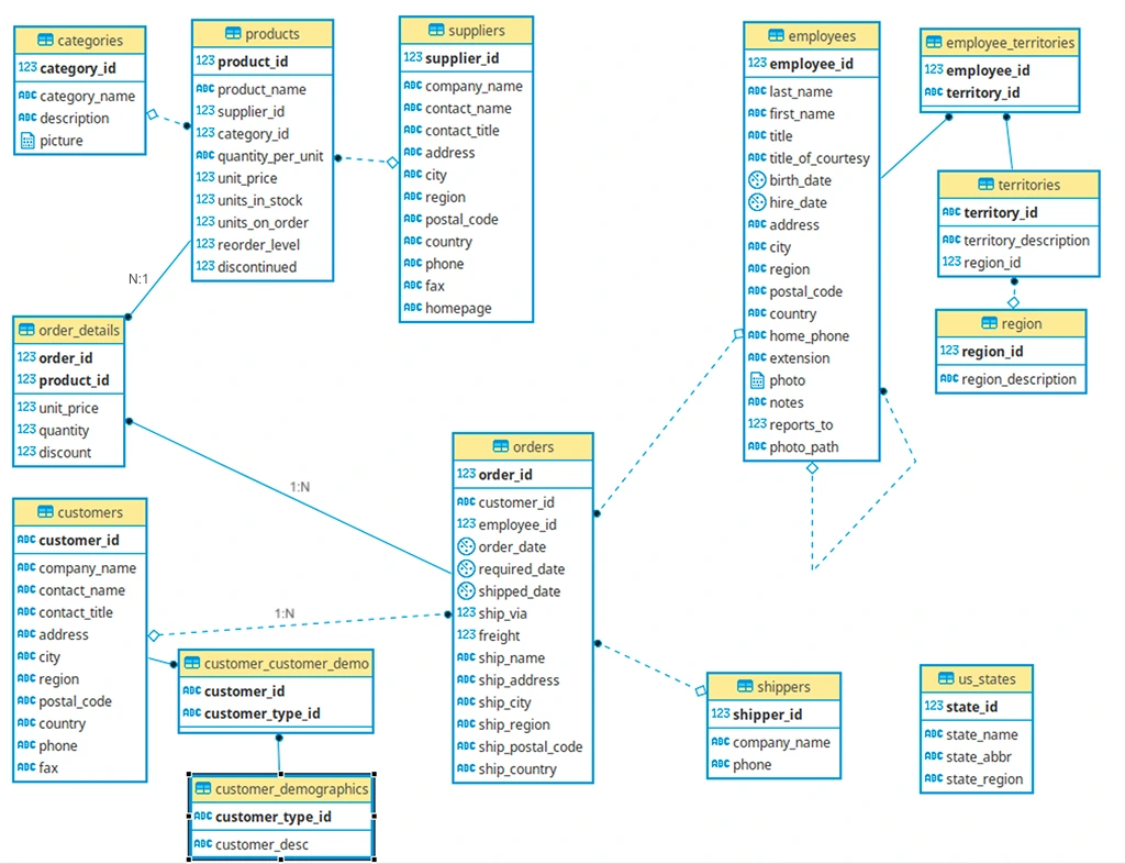
6.3. Reading the Northwind ERD
Let’s consider Figure 1 to examine the key relationships in Northwind:
6.3.1. ERD Symbols Reference
You can use tools like DBVisualizer or LucidChart to create such ERDs. When viewing ERDs, you’ll see these common symbols:
| Symbol | Meaning |
|---|---|
| (PK) | Primary Key — uniquely identifies rows |
| (FK) | Foreign Key — references another table’s PK |
| Line/Arrow | Relationship between tables |
| 1 or │ | “One” side of relationship |
| ∞ or crow’s foot | “Many” side of relationship |
6.3.2. Relationship types in Northwind:
- 1:N (One-to-Many):
customerstoorders(one customer, many orders) - N:1 (Many-to-One):
orderstocustomers(many orders, one customer) - N:M (Many-to-Many):
productstoorders(throughorder_detailsjunction table)
6.3.3. Core Transaction Flow:
customers → orders → order_details → products
Example relationship breakdown:
					┌─────────────────────┐
│     customers       │
├─────────────────────┤
│ customer_id (PK)    │ ← CHAR(5) "ALFKI", "BONAP"
│ company_name        │
│ contact_name        │
│ city                │
│ country             │
└─────────────────────┘
          │
          │ 1:N relationship (one customer, many orders)
          ▼
┌─────────────────────┐
│      orders         │
├─────────────────────┤
│ order_id (PK)       │ ← INTEGER (10248, 10249...)
│ customer_id (FK)    │ → references customers.customer_id
│ employee_id (FK)    │ → references employees.employee_id
│ order_date          │
│ ship_city           │
│ freight             │ ← shipping cost
└─────────────────────┘
          │
          │ 1:N relationship (one order, many line items)
          ▼
┌─────────────────────┐
│   order_details     │
├─────────────────────┤
│ order_id (PK, FK)   │ → references orders.order_id
│ product_id (PK, FK) │ → references products.product_id
│ unit_price          │
│ quantity            │
│ discount            │
└─────────────────────┘
          │
          │ N:1 relationship (many items, one product)
          ▼
┌─────────────────────┐
│     products        │
├─────────────────────┤
│ product_id (PK)     │ ← INTEGER (1, 2, 3...)
│ product_name        │
│ supplier_id (FK)    │ → references suppliers.supplier_id
│ category_id (FK)    │ → references categories.category_id
│ unit_price          │
│ units_in_stock      │
└─────────────────────┘
Key observations:
- Composite Primary Key in order_details:
- order_id + product_id together uniquely identify each row
- This makes sense: “Order 10248 contains Product 11” is unique
- Neither column alone is unique (orders have multiple products, products appear in multiple orders)
- Customer IDs are CHAR(5), not integers:
- Examples: “ALFKI”, “BONAP”, “BOTTM”
- This is a business decision (memorable codes vs sequential numbers)
- Still functions as primary key (unique, non-null)
- Orders table has multiple foreign keys:
- customer_id → who placed the order
- employee_id → who processed the order
- ship_via → which shipping company (references shippers)
- Products link to two dimension tables:
- category_id → what type of product (Beverages, Dairy, etc.)
- supplier_id → who supplies it
6.3.4. Business Questions Enabled by These Relationships
This schema structure allows analysts to answer:
| Business Question | Tables Needed | Relationship Path |
|---|---|---|
| “Who are our top 10 customers by revenue?” | customers, orders, order_details | customers → orders → order_details (sum revenue) |
| “Which products are best-sellers?” | products, order_details | products ← order_details (count quantities) |
| “Which categories generate most profit?” | categories, products, order_details | categories ← products ← order_details (sum revenue) |
| “Which employees close the most orders?” | employees, orders | employees ← orders (count orders) |
| “Which suppliers provide our top products?” | suppliers, products, order_details | suppliers ← products ← order_details |
| “Which countries have the most customers?” | customers | customers (group by country) |
The relationships make these analyses possible. Without foreign keys, you couldn’t connect orders to customers or products to categories.
6.4. Star Schema vs. Snowflake Schema: Database Design Patterns
Now that you understand facts and dimensions, let’s examine how they’re organized. Two patterns dominate analytical database design:
6.4.1. Star Schema: Simple and Fast
Structure:
- One central fact table
- Dimension tables connect directly to the fact table
- Looks like a star (fact in center, dimensions radiating outward)
Visual representation:
					┌──────────┐
    │ customer │
    └──────────┘
         │
         ▼
    ┌──────────┐      ┌──────────┐     ┌──────────┐
    │ employee │◄─────┤  ORDERS  │────►│ shipper  │
    └──────────┘      │  (FACT)  │     └──────────┘
                      └──────────┘
                           ▲
                           │
                      ┌──────────┐
                      │ product  │
                      └──────────┘
Characteristics:
- Simple joins: Fact → Dimension (only 2 tables)
- Fast queries: Fewer joins = better performance
- Some redundancy: Dimensions may contain duplicate data
- Denormalized: Prioritizes query speed over storage efficiency
Example query path:
					-- "What's total revenue by customer?"
SELECT customers.company_name,
       SUM(order_details.quantity * order_details.unit_price)
FROM order_details
JOIN orders ON order_details.order_id = orders.order_id
JOIN customers ON orders.customer_id = customers.customer_id
GROUP BY customers.company_name;

-- Only 3 tables, 2 joins → FAST
- Most analytics projects (default choice)
- When query performance is priority
- When data volumes aren’t extremely large
- When business users need to write their own queries (simpler to understand)
6.4.2. Snowflake Schema: Normalized and Efficient
Structure:
- One central fact table
- Dimension tables connect to sub-dimension tables
- Looks like a snowflake (branching structure)
Visual representation:
					`
                    ┌──────────┐
                    │ category │
                    └──────────┘
                         ▲
                         │
┌──────────┐        ┌──────────┐
│ supplier │◄───────┤ product  │
└──────────┘        └──────────┘
                         ▲
                         │
                    ┌──────────┐      ┌──────────┐
                    │  ORDERS  │◄─────┤ customer │
                    │  (FACT)  │      └──────────┘
                    └──────────┘           ▲
                         ▲                 │
                         │            ┌──────────┐
                    ┌──────────┐      │   city   │
                    │ employee │      └──────────┘
                    └──────────┘           ▲
                         ▲                 │
                         │            ┌──────────┐
                    ┌──────────┐      │ country  │
                    │ territory│      └──────────┘
                    └──────────┘
                         ▲
                         │
                    ┌──────────┐
                    │  region  │
                    └──────────┘
Characteristics:
- Complex joins: Fact → Dimension → Sub-dimension (3+ tables)
- Slower queries: More joins = reduced performance
- Less redundancy: Each piece of data stored once
- Normalized: Prioritizes storage efficiency over query speed
Example query path:
					-- "What's total revenue by product category?"
SELECT categories.category_name,
       SUM(order_details.quantity * order_details.unit_price)
FROM order_details
JOIN products ON order_details.product_id = products.product_id
JOIN categories ON products.category_id = categories.category_id
GROUP BY categories.category_name;

-- 3 tables, 2 joins
-- But categories is a sub-dimension of products → Snowflake characteristic
When to use snowflake schema:
- Very large databases (billions of rows) where storage cost matters
- When data updates are frequent (less redundancy = easier updates)
- When data integrity is critical (normalization prevents inconsistencies)
- When query performance can be optimized with indexes and caching
6.4.3. Why Schema Design Matters: Real Business Impact
Scenario: E-commerce company analyzing sales
Star schema approach:
					Query: "Top 10 customers by revenue"
- Join: order_details → orders → customers
- Execution time: 0.3 seconds
- Easy for business analysts to write
Snowflake schema approach:
					Query: "Top 10 customers by revenue in each city category"
- Join: order_details → orders → customers → cities → city_types
- Execution time: 2.1 seconds
- Requires understanding of complex relationships
The trade-off:
- Star = Speed + Simplicity but uses more storage
- Snowflake = Efficiency + Integrity but requires more complex queries
In practice: Most modern analytical databases use hybrid approaches (like Northwind), combining star characteristics for common queries with selective normalization where it makes sense.
6.4.5. Northwind Schema Classification: Hybrid Star-Snowflake
The Northwind database primarily follows a star schema pattern, though with some snowflake characteristics.
Evidence of star schema:
Fact table: order_details
- Contains metrics (quantity, unit_price, discount)
- Links to dimension tables via foreign keys (order_id, product_id)
Dimension tables surrounding the fact:
orders(order information) — connects directly to factproducts(product information) — connects directly to factcustomers(customer information via orders) — 1 hop from factemployees(employee information via orders) — 1 hop from fact
Simplified star view:
					`
         categories
              │
              ▼
suppliers → products
              │
              ▼
         order_details ← orders ← customers
         (FACT TABLE)       ▲
                            │
                       employees
Snowflake characteristics:
The products dimension doesn’t stand alone—it has sub-dimensions:
products→categories(product types)products→suppliers(product sources)
This creates a “snowflake” branch:
					order_details → products → categories
                         → suppliers
Similarly, the employees dimension has sub-dimensions:
orders → employees → employee_territories → territories → region
6.4.6. Classification: Hybrid (Star with snowflake elements)
Why this design was chosen:
-
Common queries are fast (star structure):
- “Total sales by product” = 1 join (order_details → products)
- “Sales by customer” = 2 joins (order_details → orders → customers)
-
Data integrity is maintained (snowflake branches):
- Product categories stored once (no duplication)
- Supplier information centralized
- Changes to category names update everywhere automatically
-
Storage efficiency where it matters:
- Category table has only 8 rows (Beverages, Condiments, etc.)
- Storing category names in every product row would waste space
- Normalizing this relationship makes sense
Why this matters for analysis:
- Simple queries (e.g., “total sales by product”) = fast (star structure: 1 join)
- Complex queries (e.g., “sales by category and supplier”) = slightly slower (snowflake branches: 2-3 joins)
- Data integrity = high (normalized design prevents duplication and inconsistencies)
6.4.7. How to Identify Schema Patterns
Steps to analyze any database schema:
1. Find the fact table(s)
-
- Look for transaction/event data (orders, sales, shipments)
- Contains metrics (quantities, amounts, counts)
- Usually has multiple foreign keys
- In Northwind:
order_details(has quantity, unit_price, discount)
2. Identify dimension tables
-
- Contain descriptive information (who, what, where, when)
- Referenced by fact tables via foreign keys
- Examples: customers, products, employees, time
- In Northwind: products, customers, employees, shippers, categories, suppliers
3. Check for sub-dimensions
-
- Do dimension tables link to other dimension tables?
- Yes = snowflake characteristics
- No = pure star schema
- In Northwind: products → categories, products → suppliers (snowflake)
4. Count the “join distance”
-
- How many tables between fact and final dimension?
- 1 join = star schema
- 2+ joins = snowflake schema
Northwind example:
- Fact (order_details) → Product = 1 join (star)
- Fact (order_details) → Category = 2 joins via Product (snowflake)
- Fact (order_details) → Customer = 2 joins via Orders (snowflake)
7. Creating a Data Dictionary
A data dictionary is documentation that explains what each table and column contains. It’s essential for:
- Onboarding new team members
- Ensuring consistent understanding across teams
- Supporting your future self when you return to a project months later
7.1. What to Include
- Entity Relationship Diagram
- For each table:
-
- Table name and purpose
- Fact or Dimensions information
- Column names, data types, and descriptions
- Primary and foreign keys
- Constraints (e.g., NOT NULL, UNIQUE)
- Links to / Links from
- Sample values (if helpful)
7.2. Example Data Dictionary Entry: Northwind Customers Table
Table: customers
Purpose: Stores customer company information including contact details and addresses for B2B sales tracking.
| Column | Data Type | Description | Constraints | Sample Values |
|---|---|---|---|---|
customer_id |
CHAR(5) | Unique 5-character customer identifier code | PRIMARY KEY | ALFKI, BONAP, BOTTM |
company_name |
VARCHAR(40) | Legal customer company name | NOT NULL | Alfreds Futterkiste, Bon app’, Bottom-Dollar Markets |
contact_name |
VARCHAR(30) | Primary contact person at customer company | Maria Anders, Laurence Lebihan | |
contact_title |
VARCHAR(30) | Job title of contact person | Sales Representative, Owner, Marketing Manager | |
address |
VARCHAR(60) | Street address of customer | Obere Str. 57, 12 rue des Bouchers | |
city |
VARCHAR(15) | City where customer is located | Berlin, Marseille, London | |
region |
VARCHAR(15) | State/province/region (NULL for countries without regions) | NULL allowed | NULL, OR, BC |
postal_code |
VARCHAR(10) | Postal/ZIP code | 12209 |
Summary
You’ve now learned the structural foundations of relational databases:
- Database structure fundamentals: Tables, rows, columns with strict data types; primary keys (unique identifiers) and foreign keys (table relationships); indexes for query performance optimization
- Data import methods: SQL dumps for complete databases, compressed archives (.tar/.dat files), and CSV files with AI-assisted table creation
- Schema analysis skills: Read ERDs to trace data relationships; distinguish between fact tables (transactions/metrics) and dimension tables (descriptive context); identify star schema (simple, fast) vs. snowflake schema (normalized, efficient) patterns
- Documentation practices: Create data dictionaries that document table purposes, column definitions, constraints, and relationships—essential for team collaboration and future reference
Suggested References
- Lucidchart – Guide to Entity Relationship Diagrams
- Vertabelo – ERD Tutorial
- Understand data modelling essentials including facts vs dimension tables
- Database Keys: The Complete Guide (Surrogate, Natural, Composite & More)
- An Overview of PostgreSQL Indexes
- Data Dictionary Explained
Exercise
Estimated Time to Complete: ~2 hours
Context: Setting Up Your New York Taxi Database
In this exercise, you’ll take your first step into working with a real operational dataset: The New York City Yellow Taxi Trip Records, one of the most widely used mobility datasets in the world.
This dataset is published by the NYC Taxi & Limousine Commission.
You will import the provided subset into PostgreSQL and set up the data environment you’ll use for the rest of the module.
Task 1: Download the Dataset Pack
Download the prepared zip file with New York Taxi Data. Inside, you’ll find:
-
schema_create.sql
Creates the following six tables:-
dim_date -
dim_payment_types -
dim_rate_codes -
dim_vendors -
taxi_zones -
fact_yellow_trips_raw_2025(will hold January 2025)
-
-
CSV files for:
-
dim_date.csv -
dim_payment_types.csv -
dim_rate_codes.csv -
dim_vendors.csv -
taxi_zones.csv -
yellow_tripdata_2025-01.csv
-
Note: At this stage, relationships across tables will not be obvious. This is intentional.
You will model relationships and build analytic structures in later lessons.
Task 2: Create the Schema in PostgreSQL
In pgAdmin:
-
Create a new database, e.g.,
nyc_taxi_2025. -
Run the
schema_create.sqlscript. -
Confirm all six tables are created.
To submit: Take a screenshot showing the 6 tables created in pgadmin.
Task 3: Import the Data into Each Table
Import each CSV into its corresponding table using pgAdmin’s Import/Export tool.
-
Make sure:
-
Header row is enabled
-
Encoding is UTF-8
-
Delimiter is comma
-
Data types load without modification
-
Important:
You are importing only January for now (yellow_tripdata_2025-01.csv).
You’ll import the remaining months later when they become analytically relevant.
Task 4: Verify the Fact Table Import
Run:
SELECT COUNT(*) FROM fact_yellow_trips_raw_2025;
You must get:
3,475,235 rows
If your number is different, something went wrong in the import. Fix it before continuing.
To submit: Take a screenshot of number of datapoints
Also run the same query on other tables to verify correct import of data.
Task 5: Create an ERD (Entity Relationship Diagram)
Use Lucidchart (recommended) or any ERD tool of your choice.
Your ERD should:
-
Show all six tables
-
Display all columns
-
Show primary keys where they exist
-
Leave relationships unconnected for now
(real-world raw datasets don’t arrive “nicely joined,” and modeling is a skill)
Export your ERD as a PDF or PNG.
Submission Format
Submit a single PDF containing the following screenshots:
-
Your pgAdmin table list showing all six tables.
-
Screenshot of successful row count (
3,475,235) -
Your ERD (
.pdfor.png) -
A short text file (
import_notes.txt) describing:-
Any import issues you encountered
-
How you fixed them
-
Anything unclear about the schema
-
Submission & Resubmission Guidelines
1. When submitting your exercise, use this naming format:
YourName_Submission_Lesson#.xxx
If you need to revise and resubmit, add a version suffix:
YourName_Submission_Lesson#_v2.xxxYourName_Submission_Lesson#_v3.xxx
2. Do not overwrite or change the original evaluation entries in the rubric.
Instead, enter your updated responses or corrections in a new “v2” (or later) column in the rubric for mentor review.
Evaluation Rubric
| Criteria | Meets Expectations | Needs Improvement | Incomplete / Off-Track |
|---|---|---|---|
| Database Setup & Table Creation | Successfully runs the schema SQL; all 6 tables created with correct structure and no errors. | Minor issues in table creation (e.g., typos, missing constraints) but schema largely correct. | Schema not created, or tables missing/broken. |
| Data Import Accuracy | All tables correctly populated; Yellow Taxi January data imported with 3,475,235 rows returned from COUNT(*). |
Import attempted but row count is incorrect or table partially filled. | Data not imported or import is corrupted/unusable. |
| ERD Creation (Lucidchart) | ERD includes all 6 tables, uses correct fields, shows thoughtful relationships (even if surrogate keys will be created later). | ERD submitted but missing tables or relationships are unclear/inaccurate. | No ERD submitted or diagram is unusable. |
Student Submissions
Check out recently submitted work by other students to get an idea of what’s required for this Exercise:

Contact
Talk to us
Have questions or feedback about Lumen? We’d love to hear from you.